(Segmenting) The Road Not Taken

Exploratory Data Analysis and Initial Modeling Attempts

The goal of this project was to segment and extract road pixels from 512 by 512 RGB satellite aerial images. We were given approximately 10,000 training images to train on and 2,170 test images for which our predictions will be evaluated. At first look, there was a large variety of images which ranged from highly urban (many buildings and roads), to mostly rural (many fields and not many buildings), to a mix of urban/rural areas. It was also clear that this was an unbalanced classification problem: 96% of pixels were non-road, and only 4% were roads.

Image data can be interpreted as a feature matrix based on color channels, and that image segmentation is simply a classification problem. Though the formulation appeared simple, the sheer size of the training data set coupled with our desire to produce a robust model for classification presented a difficult challenge.

Progression to Convolutional Neural Networks: the U-Net

As we could not rely on manually engineering a basis to map the information available in an image to its corresponding mask, we turned to deep neural networks to better approximate this function. Further research on effective network architectures highlighted the U-Net, a convolutional neural network, as the best performing network structure for the task of image segmentation.

This network essentially has two stages. First a series of 3x3 convolutions followed by non-linear activation functions and pooling contracts the image with the goal of feature extraction. In each subsequent layer of the "downward" pass, the number of feature maps is doubled while the image is shrunken. Once a sufficient number of feature maps have been created, the image is then expanded through 2x2 up convolutions and parameter concatenation with corresponding contraction layers until it reaches its original input size. The output is then passed through a fully connected layer with a sigmoid activation to create a segmentation map.

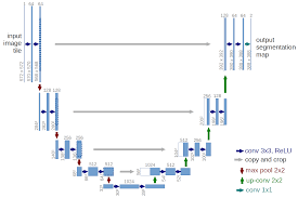
Since this method has been well explored, implementing this architecture was not difficult. What proved to be the most challenging part of creating the best model was hyper-parameter tuning. There are numerous design decisions that need be made when constructing such a network. Developing intuition about which ones will result in the model with the highest predictive power is quite difficult given the hundreds of millions of parameters present in the model, the time required for training, and our limited knowledge of the functionality of convolutional neural networks.

Fine Tuning the U-Net: Hyperparameters and Encoders

After identifying an existing architecture that had achieved comparative success in the image segmentation problem, we were eager to test its ability on our own data set and hoped to find a variation that would produce great results.

We did not anticipate the challenges that arose out of the seemingly simple task of hyperparameter tuning. We realized that in the training of such high dimensional models, it is difficult to develop intuition or a mathematical explanation on how altering a non-learned parameter can affect the model's performance. In fact, we will be the first ones to admit that our model's success was at least partially due to luck.

Introducing Pre-trained Encoders to the U-Net

The performance of our best model so far capped at around a 0.68 modified dice coefficient after post-processing. In order to increase this, we either had to improve the U-Net somehow or introduce new architectures. We looked up similar competitions in Kaggle (specifically the 2018 TGS Salt Identification Challenge and the 2015 Ultrasound Nerve Segmentation Competition for inspiration. Though many approaches were unrealistic for us in terms of compute time or complexity, many top performing contestants reported good results by integrating pre-trained encoders with an existing popular framework such as the U-Net or LinkNet. We decided to try some of these approaches with our current U-Net. Originally, we had very limited knowledge as to what these encoders actually did besides replace the classic down-sampling path of the U-Net with a more suitable path that allowed the new algorithm to either train faster, generalize better, or extract more relevant features. Upon further research, we understood the encoders as a method for creating "skip connections" over dense, complex regions in the architecture which had the effect of creating a smoother loss function, void of some of the local minima that a high dimensional model was bound to create. Using trial-and-error, we experimented with a few of these encoders such as VGG16, ResNet34, and ResNeXt50.

For all these encoders, we used weights pre-trained on the 2012 ILSVRC ImageNet dataset. We used the Python package `segmentation-models`, a Python library with Neural Networks specifically for image segmentation, to introduce these encoders to our U-Net framework. Though the images from ImageNet (which are usually ordinary photos and portraits) are vastly different from our satellite images, our reasoning for using these weights was that they provided the algorithm with better-than-random initialization values, so that the model will hopefully eventually converge to better minima than if random initialization was used.

It was clear after just a few steps within each epoch which encoders would perform the best. Notably, U-Net-ResNet34 ran extremely fast and the loss decreased quickly. In fact, the entire training process took only 5-6 hours with data augmentation and 15-20 epochs total on an AWS p2.xlarge instance, which was far faster than any model we had looked at so far. LinkNet architectures seemed to converge very slowly, so we abandoned this encoder from the get go. We believe the VGG-16 and ResNeXt50 encoders did not work as well as ResNet34 because they had a high number of parameters and no skip connections, so that overfitting was much more likely. After running a U-Net with each respective encoder until the validation loss stopped improving, we were able to see the maximum capacity of each encoder-U-Net combination. A comparison of each model is below.

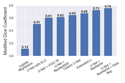
Clearly, U-Net-ResNet34 performed above and beyond all other combinations of architecture-encoders. Furthermore, this model trained very fast (around 15-30 minutes per epoch on a single Tesla K80 GPU, reaching convergence around 15 epochs) compared to the other models. Because of its high performance and speed of training, we chose the U-Net-ResNet34 as the final single model from which to ensemble and create our best set of predictions. This network was remarkably sparse, due to the skip connections (Figure 8) that allows the network to pass over unnecessary layers. This simultaneously solves the problems of too many parameters as well as the vanishing gradient issue (prevalent in networks of similar depth) as a result of having too many layers.

For future work and further improvement of the model, other architectures that we had read about in literature, such as the Stacked U-Net and Fully Convolutional Networks, may train slower but perform better than the U-Net-ResNet34.

Model Selection and Post-processing

After trying out multiple combinations of hyper parameters, implementing data augmentation, and introducing a pre-trained Res-Net encoder to our model, our result after training was the same regardless of technique used: a sigmoid output for each pixel as an associated probability of whether or not the pixel is a road. Several post processing decisions were made at this point impacting the predictive accuracy of the model.

Road Inclusion Probability and Minimum Mask Size

Given a 512x512 matrix of probabilities from any one of thegr several models we ran, we had to decide how to then convert this matrix into a proper mask that would highlight roads. We initially labeled any pixel with output probability greater than 50% as a road. Under this regime, we were frustrated by our models' inaccuracies, but failed to realize that these could in part be because of a low threshold value.

Looking at the images and corresponding masks in the training set, we realized that roads comprise a generally small proportion of the image. In fact, on average only 4% of pixels were roads (Figure 9). As a result, we hypothesized that if we increased the probability threshold when converting output to mask, i.e. required the model to be more confident when making a road classification, our accuracy would increase.

Based on the competition metric, we also introduced the idea of a minimum mask size as another post-processing step. The Dice Coefficient greatly penalizes false positives, or pixels classified by the model as roads that are not roads, when the true mask size is very low. Once we had thresholded the output probabilities, we examined each prediction to see the number of encoded roads in the predicted mask. Given that there are 512x512 pixels in a mask, we decided that there should be base minimum number of pixels classified as roads in a mask for us to find a sweet spot with the competition metric.

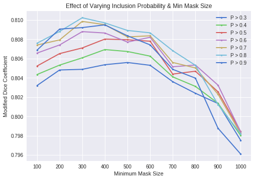
To find the optimal pixel probability and minimum mask size, we ran a simple grid search using our best model, the U-Net with a pre-trained Res-Net encoder, on training data and their true masks. We generated predictions for the first 3000 images using minimum mask sizes from 100 to 1000, and pixel probability cutoffs ranging from 0.3 to 0.9 in increments of 0.1. For each of the predictions, we compared the modified dice coefficient. The results are seen in Figure 10, and we found that a minimum mask size of 400 and inclusion probability of 0.8 produced the best dice coefficient. We used these thresholds in predictions for single models. We applied this technique to ensembles of models as well, though because the variance of an ensemble of models is lower in general, we used a probability cutoff of 0.5 and a minimum mask size of 300 for that case specifically.

Final Model

Below is a comparison of a prediction from the U-Net with a pre-trained ResNet34 encoder (right) with predictions from the classic U-Net (left), our very first model. U-Net-ResNet34 is better able to capture nuances in the image data, close road segments more successfully, and ignore random noise, when compared to the U-Net.

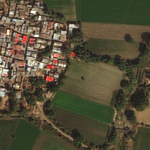
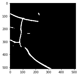
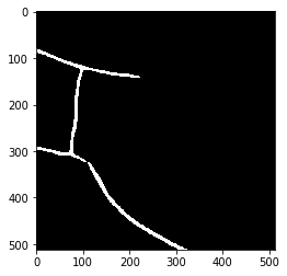
It is clear for some images, that the U-Net-ResNet34 predicts very well. This applies mostly to images with very obvious roads, of a single color, with clear edges (no shrubs or greenery obstructing the road's edges). Some cases in which our model did not do very well include narrow dirt roads, parts of images where we humans could not even confidently classify as being a road or not, and field lines in rural areas that were mistaken to be roads due to their structure. We also noticed that the algorithm had problems "closing" roads by connecting them together; this problem was more evident in areas of high classification uncertainty.

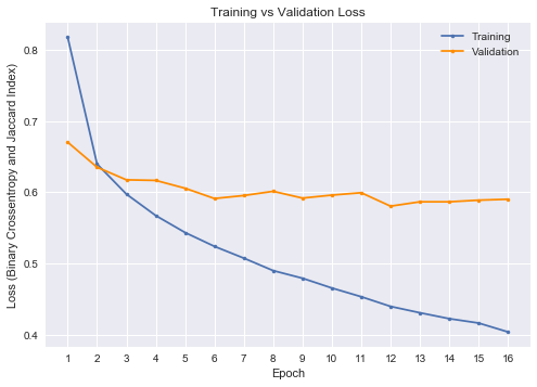
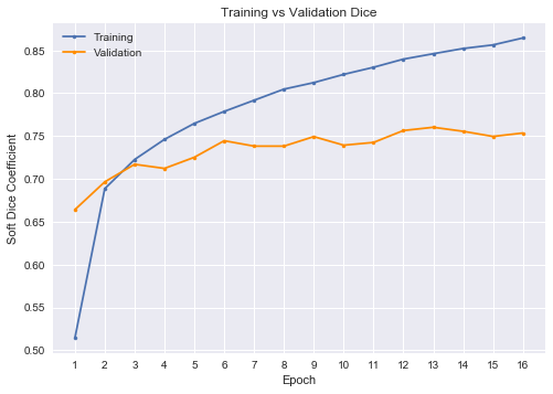
We also include a plot of training and validation loss and dice coefficient over time (epochs) for the U-Net-ResNet34 with data augmentation. The training loss and dice coefficient continue to decrease, but validation loss and dice appear to have stagnated. It's clear that the algorithm is learning a great deal about the training set, but that learning is not translating very well past the first epoch to new images. Perhaps having learning that generalizes better to new images is not possible (or very difficult), but given more time and computing resources we would have experimented with different architectures.

As a final step to improve prediction accuracy, we ensembled two models by averaging their sigmoid outputs together. Specifically, we trained one U-Net-ResNet34 without data augmentation, saved the results, trained a second U-Net-ResNet34 (this time WITH 5000 data-augmented images added manually to the training set), and saved the second set of results. We then averaged the resulting probabilities together. Though the model with data augmentation clearly performs better, ensembling it with the model without data augmentation reduces the overall variance of the sigmoid probabilities and thus gives higher accuracy.

Conclusion

This project represents our gradual improvement in understanding machine learning methods both simple and complex as applied to an image segmentation problem. At the beginning of the project, when we had minimal knowledge of convolutional neural networks, we applied what we did know of machine learning (namely logistic regression and K-means clustering) to the problem and achieved nontrivial, though not very accurate, results.

As we learned more about CNNs, we were able to implement a basic deep network called the U-Net with very promising results. We gradually improved the algorithm through multiple small steps and finally achieved an improvement of over 10% accuracy over our original U-Net.

Our final model utilizes a self-tuned U-Net-ResNet34, and achieved a modified dice coefficient of over 0.76 on both the public and private leader boards. We placed 8th on the public Kaggle board, and 10th on the private board. We have learned a lot through this project, mostly through both trial and error and connecting what we learned in class to new methods discovered through research on similar problems.

Though our model exceeds the performance of a simple U-Net, there is ample room for improvement. Future work would include ensembling (averaging the sigmoid output from multiple different models, and not our "pseudo"-ensembling of two essentially identical models). We were not able to train a model with an entirely different architecture than the U-Net-ResNet34 and still produce a comparable validation accuracy. Indeed, our second-best performing model was the Extended U-Net which capped at a much lower 0.68 dice. We were worried about ensembling our U-Net-ResNet34 with a model that performed much worse, thinking it would lower accuracy overall.

We also would have liked to experiment with additional image morphology, in particular designing kernels that could be used for our specific application. The Opening operation that we had applied was limited to single, isolated pixels and would not catch, for example, an island of two neighboring pixels. We also would have liked to spend time exploring other architectures such as the LinkNet, PSPNet, etc., in depth, and adding a decaying learning rate to allow for a coarse-to-fine search in parameter weights. Finally, though we had experimented with test time augmentation (TTA), it ultimately failed and produced worse results than originally. We coded our own TTA, which involved 3 basic transformations (left/right flip, up/down flip, and a combined flip) then averaged the results after de-transformation. Perhaps doing TTA from an existing Python package would have produced better results.

In conclusion, considering that at the beginning of this project we had little to no knowledge of deep neural networks or how to even tackle such a complex problem, we were able to develop and tune a model that not only adequately extracted roads from satellite images, but also greatly outperformed a basic U-Net. Now, we are finally able to relate to the saying that "training neural networks is hard."